Background
I think we can all agree on the following facts of life: an unsupervised self-study class, the moment the teacher's footsteps fade down the corridor, immediately becomes the closest thing to a livestock market that a school building has ever hosted. Then, the second those same footsteps return — never mind that the teacher is still a solid thirty seconds away and probably looking for their lanyard — the room achieves a level of collective silence usually reserved for the funerals of people we didn't much care for.
But here's the bit that's genuinely interesting, the bit that kept me up at night for longer than I'd like to admit: sometimes you don't even need the teacher to actually turn up. In what feels like two heartbeats, the entire room goes quiet. No one shouts "the teacher's coming." No one rings a bell. There's no visible signal at all. It's as if fifty-odd people have signed a binding contract, in triplicate, agreeing to shut up at exactly the same moment. This "spontaneous silence" thing — well. I find it rather fascinating. (I also find it vaguely sinister, but we'll come back to that.)
Group Tacit Understanding and the Power of Suggestion
Humans are, fundamentally, insufferably social creatures. The second one person stops talking, everyone else immediately starts to wonder why they stopped talking, and then they stop talking too, and before you know it you've got a chain reaction of silence with no apparent cause. (I used to think this was unique to humans. Then I watched a colony of ants do something similar with a dropped sandwich, and I had to reassess.)
There's also the small matter of psychological suggestion. Someone whispers "the teacher's coming" — or just raises a single, slightly dramatic finger to their lips — and everyone immediately drops into what can only be described as "Lesson Mode." Pavlov's dogs had nothing on us. They salivated at bells. We freeze at the sound of a slightly familiar lanyard clinking in the corridor.
A Quick Detour Through Complex Systems Theory
Look, I know what you're thinking. "Self-study silence, fine, but is there any way to make this sound vaguely academic?" The answer, of course, is yes, because we can model the classroom as a complex adaptive system. Each student is a node. Each interaction is an edge. The system as a whole does the whole "emergence" thing, where the macro behaviour is something none of the individual nodes ever signed off on. Nobody in the class decides "we will now be silent." The silence just happens. It's like an ant colony solving a sudoku — no single ant understands sudoku, but together, they manage.
A complex adaptive system, for anyone who's been living under a very comfortable rock, is just a system made up of lots of little agents who keep interacting, learning, and adapting. They're not isolated; they're tangled up with each other in a way that makes the whole thing behave like a single, slightly confused organism. The system self-organises, reaches some kind of dynamic equilibrium, and generally behaves in ways that no individual component was briefed on.
"Emergence" is the magic word here. It refers to those delightful properties that pop up at the system level and absolutely do not exist at the individual level. An ant, taken on its own, is a creature of modest intellectual achievement. Put a million of them together and they will build you a functional ventilation system for their nest. (Honestly, what are the rest of us even doing with our time?)
The Modelling Bit
Chatting away during a self-study lesson is — let's be honest, between you and me — a small but distinctively forbidden activity. Years of being told that rules exist, that rules are good, that rules are there for a reason, etc., etc., have left us with a permanent, low-grade guilt reflex. We sit there, supposedly working, but our souls are sweating.
Psychologically speaking, the teacher represents Authority. Authority represents Order. Order represents the part of our lizard brain that remembers what happens if we don't behave. The instant we register that the teacher has materialised, the subconscious takes over, and we become, essentially, well-trained lab rats. Pavlov would have had a field day. (And his dogs, presumably, a field day of their own.)
The students, meanwhile, are all in a state of high alert. Every sense is dialled up to eleven. We're scanning the doorway, the windows, the slightly off-kilter angle of light on the corridor floor. Animal behaviour scientists have a name for this. They call it the "Freeze Response" — that delightful cocktail of acute terror and the sudden inability to move your legs. It is, in the evolutionary sense, the most sensible thing a prey animal can do, right up until a predator walks past and decides you look like lunch.
Now: imagine one student, somewhere in the middle of the room, catches a glimpse of a reflection in the window and decides, with the calm confidence of someone who has been told off many times, that the teacher is on the way. This student goes quiet. The overall classroom volume drops by a fraction. That fraction is enough to push the volume below the "freezing threshold" of a second student, who also goes quiet. The volume drops further. A third student freezes. A fourth. A fifth. The feedback loop tightens. The classroom, which seconds ago resembled a stadium during extra time, is suddenly so quiet you can hear the existential dread of the student in the back row.
And nobody has actually seen the teacher. (Reader, they never do.)
Methods and Results
A One-Dimensional Cellular Automaton
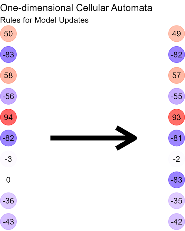
What better way to model fifty hormonal teenagers than with a one-dimensional cellular automaton? (Answer: there is no better way. Don't @ me.) A cellular automaton is a row of cells, each in some state, each updating according to a rule, every time step. Simple. Elegant. Just like a classroom full of teenagers, in other words.
In our model, the classroom is a line of fifty cells. Each cell is a student. Each student is either "talking" or "listening." We give each cell a numeric value: positive means they're talking, negative means they're listening. If a value hits zero, the student has just finished a sentence and is, briefly, in a state of contemplative silence — at which point we re-roll the dice and assign a new random value between -100 and +100.
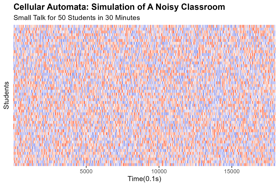
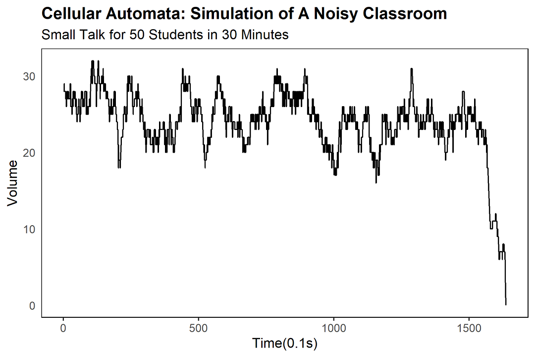
We set the time step at 0.1 seconds, and we let a single sentence last up to 10 seconds. So a student who starts with a value of +100 will, after 100 time steps, drop to zero, having said their piece, and then re-randomise. The result, after a few minutes, is a beautifully chaotic pattern of red and blue.
We run 18,000 time steps, which corresponds, in human time, to about thirty minutes of self-study. (This is, coincidentally, exactly the maximum attention span of the average Year 10 student on a Friday afternoon. I have done the research. I was the Year 10 student on the Friday afternoon.)
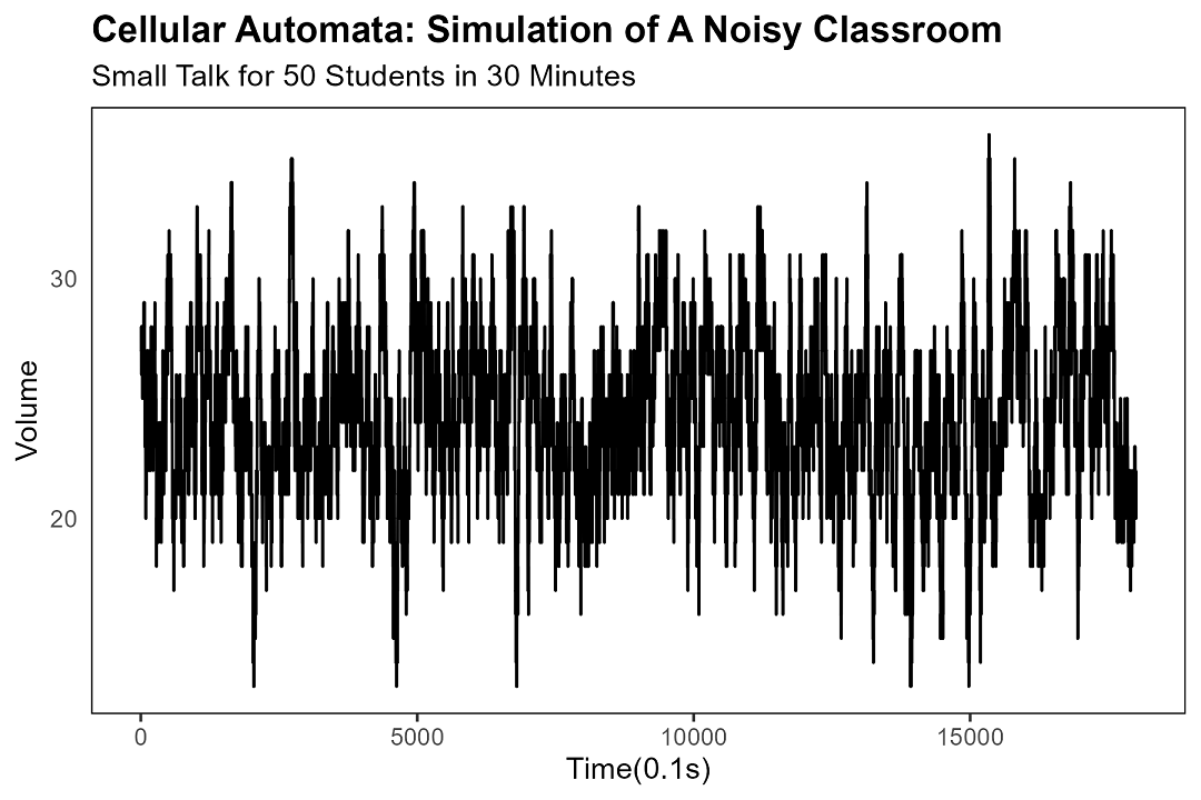
To measure how loud the classroom is, we count the number of students currently mid-sentence. Because nothing says "rigorous quantitative analysis" like counting heads in a line.
The Freeze Response
Now, let's add the bit that makes the model actually interesting — namely, the fact that students have a complicated relationship with their teachers that can broadly be described as "traumatic." For each student, we introduce a new variable: their minimum freezing volume, or x. This is the number of students that need to be talking before this particular student starts to suspect something is afoot and goes quiet. Some students have what can only be described as a large psychological shadow area — they panic the moment the noise drops below seventeen other voices. Others, the brave little toasters, won't freeze until it's just them and one friend still chatting, at which point they think, "Huh, is it just us?"
So: if, in the previous time step, the number of students talking was less than this student's x, we set the student's state to -10 for the next ten time steps, which represents one second of stunned, watchful silence. Otherwise, we proceed with the original rule.
Each time a student freezes, the volume drops, which can then trip the threshold of another student, who freezes, and so on. This is — congratulations, you've been paying attention — the feedback loop that produces "spontaneous silence."
In the simulation, spontaneous silence strikes at around 160 seconds, give or take. (In a real classroom, the timing varies. Sometimes it takes five minutes. Sometimes it takes five seconds. Sometimes it doesn't happen at all, and someone ends up in detention.)
A Note on Parameters
Whether the whole "group tacit understanding" thing actually happens depends, in a complicated and non-linear way, on the size of the system. Small tweaks to the initial parameters can produce wildly different outcomes. So we have to be careful. (This is, broadly, the same lesson that climate scientists have been trying to teach us for the last thirty years. We didn't listen then, and we probably won't listen now.)
In our model, each cell starts with a random state, and the only thing we vary, systematically, is each student's minimum freezing volume x.
To keep the model at least vaguely tethered to reality, we set the minimum x — the threshold for the most insensitive student — at 3. So that particular student won't freeze until there are only three other people talking. The maximum x is harder to pin down, so we have to explore the parameter space the fun way: by running lots of simulations and seeing what happens.
With xmin = 3 and xmax = 17, we ran 10,000 simulations. For each, we recorded the sum of the freezing volumes of all fifty students (call it Sx = Σ xi) and the time at which spontaneous silence first occurred (up to a maximum of 18,000 time steps, or thirty minutes).
| Estimate | Std.Error | t | P | Sig. | |
|---|---|---|---|---|---|
| (Intercept) | 6.0676688 | 0.0829139 | 73.18 | <2e-16 | *** |
| $S_x$ | -0.0056127 | 0.0001652 | -33.97 | <2e-16 | *** |
Table 1: Linear regression of spontaneous silence time against the sum of the students' psychological shadow areas.
We then increased xmax from 15 to 19, ran a few thousand simulations at each value, and counted how often spontaneous silence occurred within the thirty-minute window. We fit a logistic regression to the data and got the following:
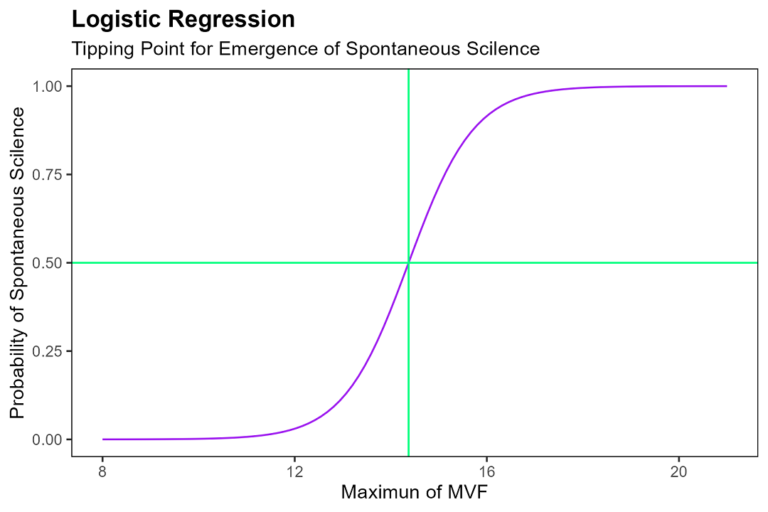
Figure 6: Logistic regression model y = [1 + exp(-1.463x + 21.019)]-1 and its threshold.
What this is telling us, in plain English, is roughly the following: when the number of students currently talking drops below a critical value, a chain reaction of freezing kicks in, and the classroom goes quiet — fast. In a thirty-minute self-study lesson, if the maximum freezing volume among the fifty students crosses a tipping point of about 14, spontaneous silence becomes a lot more likely. Above 19, you can basically bet your pocket money on it.
In Closing
"Freeze, Flight, Fight" — the three Fs — are pretty much the universal response package for any creature, mammal or otherwise, that has the misfortune of encountering something that wants to eat it. Studies have shown that doing nothing at all is, paradoxically, often the smartest move for a prey animal. This is because the visual cortex and retinas of mammalian predators have, over millions of years, become extremely good at detecting motion. So the rabbit that stops, listens, and stares into the middle distance is, statistically speaking, a rabbit that's going to live long enough to be eaten another day. (Not the cheeriest motivational poster, I know. But then, biology rarely is.)
Out there in the wider world, there's a charming English expression for this particular flavour of sudden quiet: "An angel passing by." I find this unbearably poetic, in the way that only things you don't really believe in can be.
Maybe — and I realise this is a stretch — maybe some of those teachers actually were angels. It took me an unreasonably long time, but I eventually came to appreciate just how much they did. I only realised, sometime in my twenties, that the strict hand of a good teacher is one of the few things standing between a teenager and his or her own worst impulses. We weren't built for self-discipline. We were built for peer pressure, sugar, and the quiet terror of being told off in front of the class.
Looking back, the people who wandered into your life for a year, maybe two, and then wandered out again — and who genuinely, sincerely wanted the best for you — are rarer than they ought to be. The older I get, the fewer of those people I seem to find. If you happen to know where any of them are, please do pass on my thanks. They probably saved your life, or at the very least your GPA.
That said, there is always, always, going to be a sacrificial lamb. Someone has to take the detention so the rest of us can continue the pretence that we are, in fact, model students. Don't, as the saying goes, take the mickey out of the teacher. Even the most angelic of us has their limits.
Appendix I: Cellular Automaton Implementation
i <- 1
timestep <- 1
timeout <- 18000
students <- 50
t0 =  round(runif(students, -100, 100))
ca <- cbind.data.frame(t0)
volume <- vector(mode="numeric")
volume[timestep] <- sum(ca[,timestep] > 0)
mentalshadow <- round(runif(students, 3, 19))

while(volume[timestep] != 0){
  for(i in 1:students){
    if(volume[timestep] < mentalshadow[i]){
      ca[i, timestep + 1] <- -10
      }
    else {
      if(ca[i, timestep] == 0) {
        ca[i, timestep + 1] <- sample(-100:100, 1)
        }
      else if(ca[i, timestep] > 0) {
        ca[i, timestep + 1] <- ca[i, timestep] - 1
      }
      else {ca[i, timestep + 1] <- ca[i, timestep] + 1}
    }
  }
  colnames(ca)[timestep+1] <- paste0("t", timestep)
  timestep <- timestep + 1
  if(timestep == timeout){volume[timestep] = 0}
  else{volume[timestep] <- sum(ca[, timestep] > 0)}
}
Appendix II: The Trap of Vectorised Computation
R, as anyone who has ever tried to use it for anything serious will tell you, is built for vectorised computation. Vectorised operations are, broadly speaking, much faster than the equivalent for loop, because the underlying engine is written in C, the whole vector is handed off in one go, and the interpreter gets to put its feet up. (This is, broadly, the entire sales pitch of R, and also the reason nobody ever uses R for anything where speed actually matters.)
When generating simulated data according to some rule, the natural instinct is to reach for vectorised computation (ifelse) rather than the more tedious loop. But — and this is the bit the tutorials don't tell you — vectorised computation can, if you are not paying attention, sneak in a "lockstep" trap, introducing patterns where there should be randomness, and quietly destroying the heterogeneity of your simulation.
The Anomalous Pattern of Synchronised Evolution
In our simulation, each individual's state value fluctuates within a range, following these rules:
- If the state is positive, it decreases by one each step; if negative, it increases by one.
- If the state is zero, the individual is assigned a new random value.
ifelse(state == 0, sample(new_values, 1), state ± 1)
In principle, this should preserve a healthy amount of heterogeneity. But when you implement it directly with vectorised computation, all the states change in synchrony.
set.seed(1)

ca <- data.frame('step0' = round(runif(50, min = -100, max = +100)))

for (t in 1:100) {
  ca_rule <- ifelse(ca[, t] == 0, sample(-100:100, 1),
                    ifelse(ca[, t] > 0, ca[, t] - 1, ca[, t] + 1))
  ca[,ncol(ca) + 1] <- ca_rule
  colnames(ca)[ncol(ca)] <- paste0("step", t)
}

rownames(ca) <- paste0("Student ", 1:50)
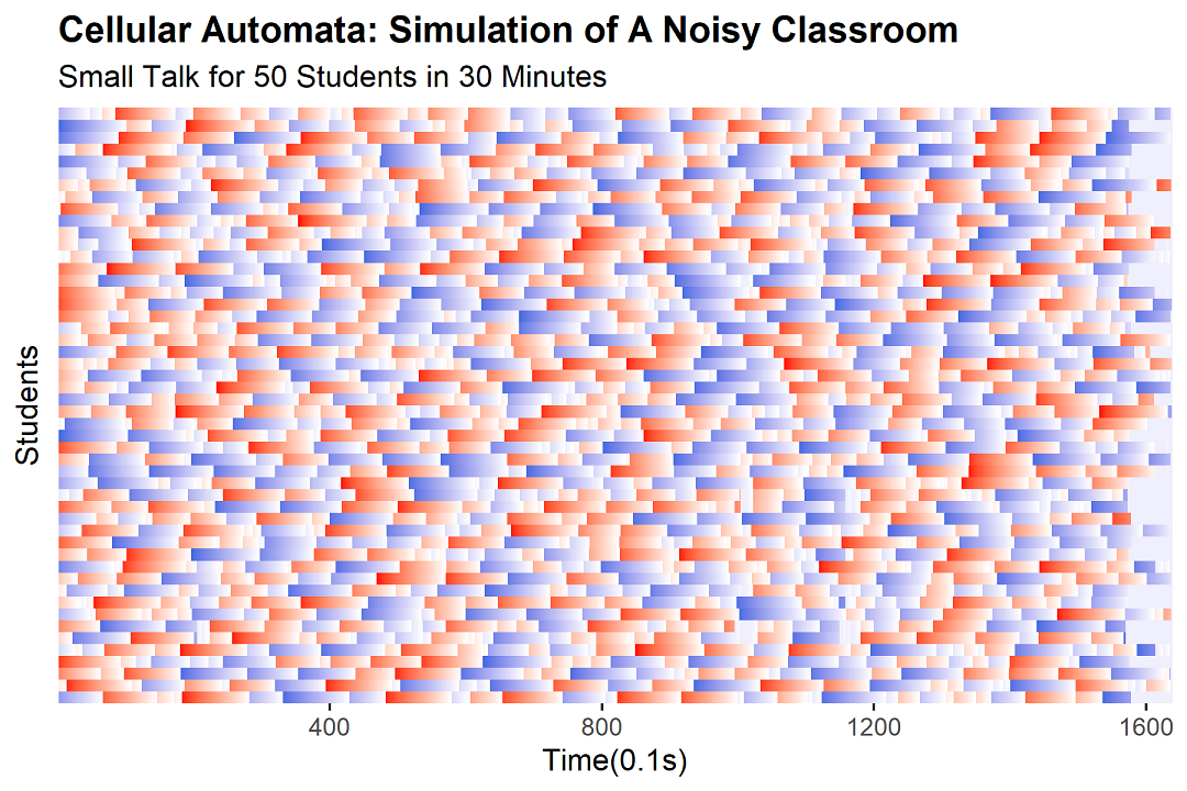
On the surface, this code appears to do exactly what we want. But the catch is that sample(-100:100, 1) generates one random number, which is then assigned to every individual that happens to have a state of zero at that time step. So if several students happen to finish their sentences at exactly the same moment — and in a synchronised system, they do, all the time — they all get the same new value, and they then proceed, in perfect lockstep, to evolve identically for the rest of the simulation. (You can see the problem. Several of them, in fact, walking in step.)
pheatmap(ca,
         cluster_rows = TRUE,
         cluster_cols = FALSE,
         show_rownames = TRUE,
         show_colnames = FALSE,
         treeheight_row = 0)
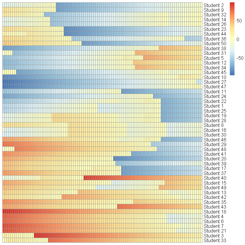
The hallmarks of this syndrome are:
- As in the figure above, certain individuals develop identical trajectories, marching in perfect lockstep.
- The heterogeneity we were promised has, in fact, vanished.
- If a large enough proportion of the population is affected, the simulation results can diverge significantly from the intended behaviour.
This is bad. This is, to use a technical term, bad. The randomness is undermined, the heterogeneity is undermined, and the simulation starts behaving in ways that bear only a passing resemblance to what you actually asked for.
How to Avoid This Disappointment
To keep the individuals properly independent, we need to make sure each one gets its own random number at each update, particularly when the state is reset. The simplest way to do this is to identify all the individuals currently sitting at zero, and then assign each one a separate random value. This still uses vectorised computation under the hood, and so it remains reasonably fast, but it doesn't have the lockstep problem.
vectorized_update <- function() {
  ca <- data.frame('step0' = round(runif(50, min = -100, max = +100)))

  for (t in 1:1000) {
    zero_indices <- which(ca[, t] == 0)
    new_random_values <- sample(-100:100, length(zero_indices), replace = TRUE)

    ca_rule <- ifelse(ca[, t] == 0, NA,
                      ifelse(ca[, t] > 0, ca[, t] - 1, ca[, t] + 1))

    if (length(zero_indices) > 0) {
      ca_rule[zero_indices] <- new_random_values
    }

    ca[, ncol(ca) + 1] <- ca_rule
    colnames(ca)[ncol(ca)] <- paste0("step", t)
  }
}
The traditional loop-based approach, by contrast, generates a fresh random number for each individual in turn, which guarantees the independence we wanted in the first place. The trade-off, of course, is that it's slow. Painfully, embarrassingly slow.
loop_update <- function() {
  ca <- data.frame('step0' = round(runif(50, min = -100, max = +100)))

  for (t in 1:1000) {
    ca_rule <- numeric(50)
    for (i in 1:50) {
      if (ca[i, t] == 0) {
        ca_rule[i] <- sample(-100:100, 1)
      } else if (ca[i, t] > 0) {
        ca_rule[i] <- ca[i, t] - 1
      } else {
        ca_rule[i] <- ca[i, t] + 1
      }
    }
    ca[, ncol(ca) + 1] <- ca_rule
    colnames(ca)[ncol(ca)] <- paste0("step", t)
  }
}
- The
ifelse()vectorised operation is implemented in C, and so is much faster than the equivalentforloop. - However, because
sample()invectorized_update()generates multiple random numbers in one call, whileloop_update()callssample()once per individual, the number of calls in the loop version is far higher. - And, separately,
which(ca[, t] == 0)finds all the zero-state cells in one operation, which is also much faster than checking them one at a time.
We would therefore expect the vectorised version to be considerably faster, and this is borne out in practice.
replicate(5, system.time(vectorized_update())["elapsed"])
0.340000000000146
0.319999999999709
0.340000000000146
0.270000000000437
0.25

replicate(5, system.time(loop_update())["elapsed"])
2.5
2.42000000000189
2.40999999999985
2.90000000000146
2.88999999999942
A simple system.time() call confirms the obvious: vectorised computation is, for large data and long simulations, drastically faster. (The loop version, in this case, takes about ten times as long. Ten. Times. I could have done this by hand. Probably.)
To summarise: vectorised computation, in R, is the right choice almost all of the time, especially when the dataset is large or the simulation is long. But when the computation involves randomness, you have to be careful — very careful — that you don't accidentally introduce a synchronised, lockstep pattern into a system that is supposed to be heterogeneous.
The trade-off, in the end, is this: pay the speed cost of a for loop, and you get genuine independence between your simulated individuals. Skimp on it, and your simulation is, at best, a passable impression of what you wanted. (And at worst, it's a PowerPoint slide waiting to happen.)